This is a synthesis of the method developed and applied in MapBiomas Soil for modeling and mapping soil properties in the Brazilian territory. The detailed description of the data, methods and algorithms will be available soon.

1. Introduction

The third collection (beta version) of MapBiomas Soil features annual soil organic carbon (SOC) stock maps for Brazil (1985–2024) at a 30 m resolution, expressed in tons per hectare (t/ha) for the top 30 cm of soil depth.

One of the new features of this collection is the expansion of the depth range for the static particle size distribution maps (percentage of sand, silt, and clay) and soil texture classes (three classification systems) up to 100 cm depth, provided in 10 cm thick layers.

The collection also introduces novel static soil stoniness maps. These maps represent the soil depth (cm) at which the volume of coarse fragments reaches 50% (dominant stoniness) and 90% (extreme stoniness), with a depth limit of 100 cm.

The maps were developed using field soil data published in the SoilData Repository (http://soildata.mapbiomas.org/) and dozens of predictor variables available in public spatial data sources. Soil property maps can be accessed through the Soil module on the MapBiomas platform (https://plataforma.brasil.mapbiomas.org/), where they can be visualized and downloaded for different territorial, environmental, and administrative areas.

Table 1. Soil property maps with 30-meter spatial resolution available in the MapBiomas Soil module for the Brazilian territory.

Soil property	Definition	Type of variable	Soil layer	Temporal resolution	Nominal year¹
Soil organic carbon stock (SOC)	Maps of SOC stocks	Continuous (stocks ranging from 0 to 255 t/ha)	0 – 30 cm	Annual	Does not apply
Particle size	Maps of sand, silt, and	Continuous	0-10, 10-20, 20-30, 30-40, 40-50, 50-60, 60-70, 70-80, 80-90 e 90-100 cm	Does not apply	1990
Texture	Maps of soil texture classes	Categorical (five, eight, and thirteen classes)	0-10, 0-20, 20-40, 0-30, 30-60, e 60-100 cm	Does not apply	1990
Stoniness	Depth maps up to stoniness thresholds: dominant (volume>50%) and extreme (volume>90%)	Continuous	0-100 cm	Does not apply	1990

2. Concept

Following the principles of digital soil mapping, soil properties are modeled using machine learning algorithms that establish statistical relationships between field-collected soil samples and predictor variables, which represent soil formation factors and processes.

Static predictor variables represent the formation factors that structure the spatial variation of soil properties. Dynamic variables, on the other hand, capture changes over time, such as climatic variations and land use and cover transformations. The statistical relationships computed by the models are used to estimate how soil properties vary across space and time, resulting in the generation of static maps and annual series for the 1985–2024 period.

The machine learning algorithms employed—Random Forest and Gradient Tree Boosting—are based on ensembles of randomized regression trees. These trees use data subsets to process statistical relationships between field observations and predictor variables. The spatial and temporal variation of soil properties is estimated based on the consensus of these trees.

The primary difference between the two algorithms lies in how the regression trees are combined. Random Forest operates with independent trees whose results are averaged. Analogously, it is as if hundreds of specialists were mapping the same area independently, with the final map being the average of their individual interpretations.

In contrast, Gradient Tree Boosting constructs trees sequentially, where each new tree aims to progressively correct the errors of the previous one. This process is akin to hundreds of specialists successively refining each other's work until reaching the final result.

3. Training samples

Soil data were sourced from various studies published in the SoilData repository (http://soildata.mapbiomas.org/)Following analysis, a selected set of studies was used for spatial modeling of soil granulometry (clay, silt, sand, and coarse fragments). These datasets encompass thousands of points across the Brazilian territory, totaling multiple soil layers up to a depth of 100 cm. Since coarse fragment data were missing for many samples, values were estimated using pedotransfer functions (PTFs). For modeling, the percentage proportions of clay, silt, sand, and coarse fragments were transformed into "additive log-ratios" (ALR) — log(sand/clay), log(silt/clay), and log(coarse fragments/clay) — a mathematical approach that enhances modeling stability and consistency.

For space-time modeling of SOC stocks, datasets were selected comprising thousands of points and soil layers. Missing bulk density values were estimated using pedotransfer functions. After quality control, suitable data were used for training the space-time SOC stock model. The SOC stock for each layer was calculated using the equation: carbon content × (1 - coarse fragments) × bulk density × layer thickness.

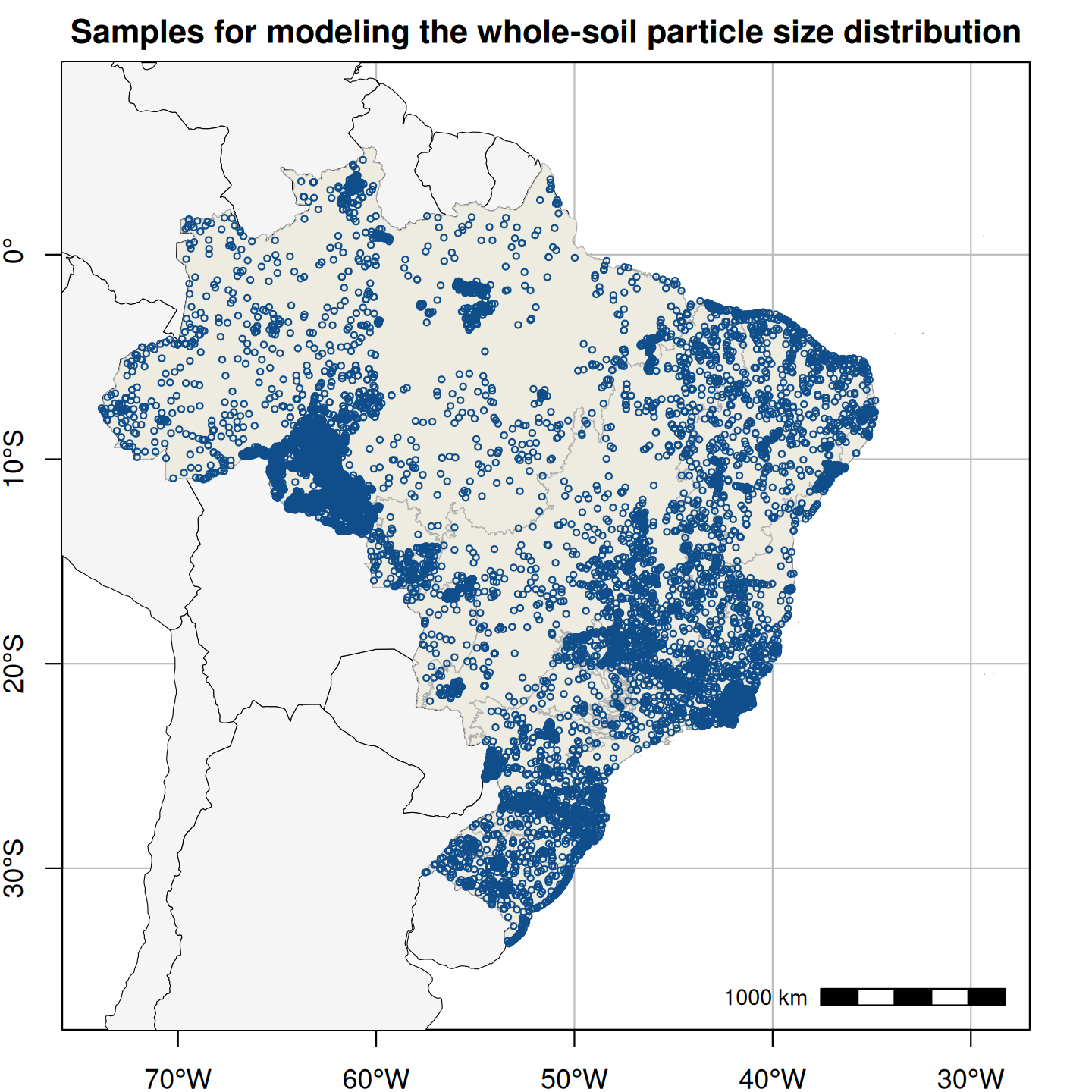
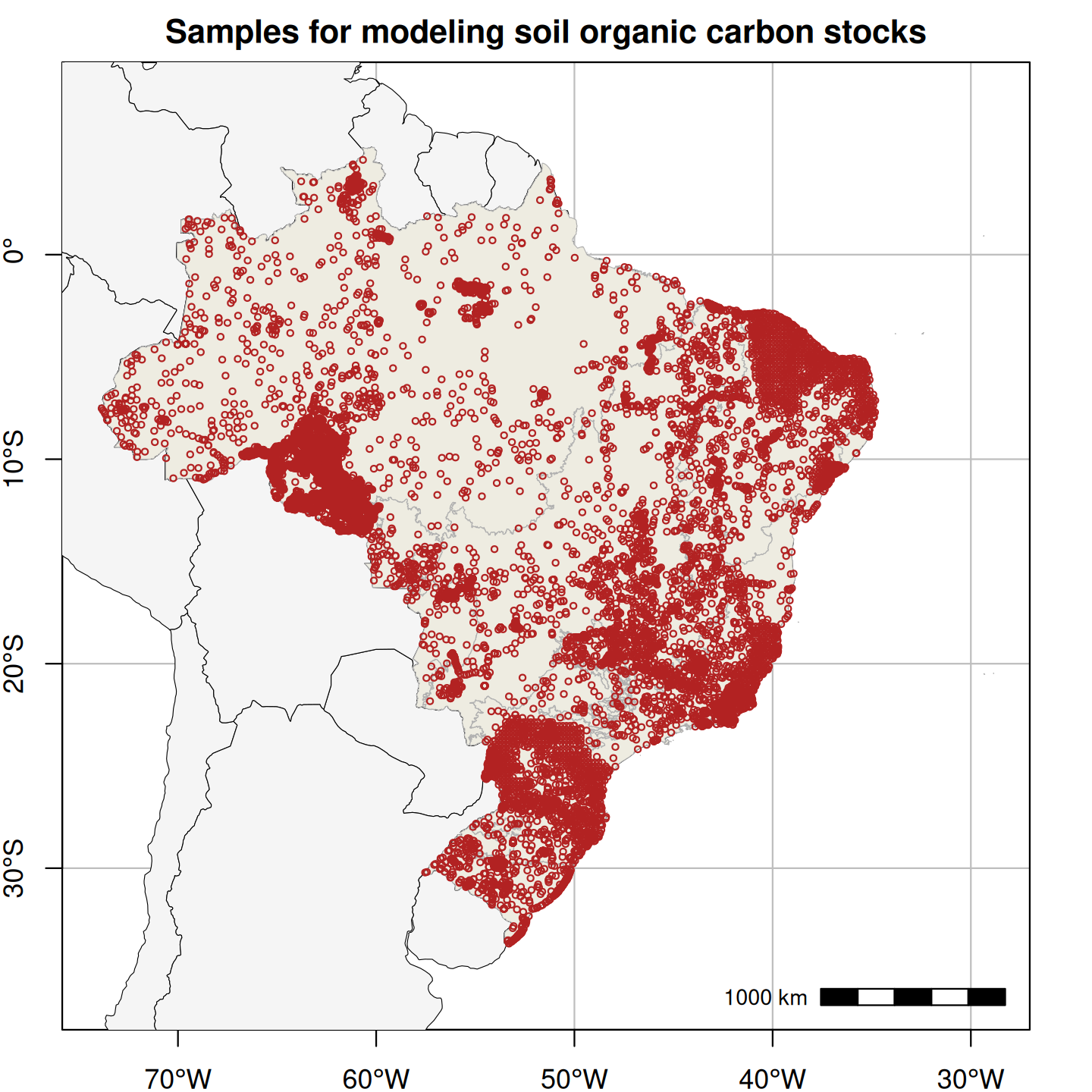
Figure 1. Spatial distribution of field-collected training samples used in the spatial modeling of soil particle size distribution (left; 15,798 points and 60,883 samples) and the spatio-temporal modeling of annual soil organic carbon stock (right; 16,013 points and 31,047 layers).

Data processing was conducted locally using R and Python, and in the cloud via Google Earth Engine. The code is available under an open license on GitHub (https://github.com/mapbiomas/brazil-soil). The data are available under the Creative Commons Attribution CC-BY license in the SoilData repository at the following links: https://doi.org/10.60502/SoilData/OXSR2N (particle size distribution) and https://doi.org/10.60502/SoilData/IUZOAK (SOC stock).

4. Predictor variables

Static and dynamic raster and vector data were obtained from open databases for all of Brazil. In Google Earth Engine, gaps were filled and the spatial resolution was standardized to 30 m.

Multi-categorical variables—including climate (Köppen), phytophysiognomy, geology, soils, and biomes (IBGE)—were converted into binary indicators to ensure algorithmic compatibility. Additionally, synthetic variables were generated by combining soil classes, parent material, and environmental compartments to capture complex pedological relationships that isolated variables could not represent.

Soil property maps were aggregated by depth (e.g., using granulometry to model carbon) and integrated with FAO/SoilGrids probabilities. Relief was represented by Geomorpho90m, while hydrology and climate dynamics were captured by statistically aggregated water layer indicators. To incorporate spatial context, geographic distances to features such as sand patches and rocky outcrops were calculated.

Vegetation indices (NDVI and EVI) from Landsat were modeled with weighted moving averages to represent long-term biomass effects on the soil. Finally, the temporal effect of land use was represented by the age evolution of each MapBiomas Land Cover 10.0 class.

Tabela 2. Some examples of static and dynamic predictor variables used in modeling soil particle size fractions (133) and annual SOC stock (126) associated with the soil state factor or change vector they represent.

Factor or vector	Predictor variable	Type of variable
Soil	Sand, silt, and clay content 0-30 cm Source: MapBiomas Solo, Collection 3.0	continuous; static
	Pedological classification (1st categorical level) Source: IBGE	categorical; static
	Probability of occurrence of soil classes Source: SoilGrids 1.0 and FAO GBSmap	continuous; static
Climate	Köppen climate classification Source: Alvares et al. (2013)	categorical; static
Hydrology; Climate change	Soil cover with water layer (presence/absence and absolute frequency) Source: MapBiomas, Collection 10.0	continuous; dynamic and static
Organisms	Classification of primary vegetation (phytophysiognomy) Source: IBGE	categorical; static
Land cover and land use persistence and chang	Age of land cover and land use class Source: MapBiomas, Collection 10.0	continuous; dynamic
	Vegetation indices such as NDVI, SAVI, and EVI Source: Landsat images	continuous; dynamic
Degradation or loss of organisms	Indicators of native vegetation degradation (distance from anthropogenic use edge) Source: MapBiomas Degradation, Collection 1.0 Beta	continuous; dynamic
	Fire occurrence indicators (cumulative occurrence; years since the last fire) Source: MapBiomas Fogo, Collection 4.0	continuous; dynamic and static
Relief	Terrain morphometric variables such as slope, compound topographic index, and elevation Source: Geomorpho90m	continuous; static
Geology	Geological classification (structural provinces) Source: IBGE	categorical; static
Territory or spatial position	Territorial classification by biome Source: IBGE	categorical; static
	Distance to spatial features (sand patches, rock outcrops)	continuous; static

5. Modeling and mapping

Training matrices for the machine learning algorithms were generated by intersecting soil sample data with predictor variables. In both granulometry and SOC stock modeling, the target layer depth was included as a predictor. The Gradient Tree Boosting algorithm was applied to the spatial (2D) modeling of granulometry, while Random Forest was used for the spatiotemporal-vertical (4D) modeling of SOC stocks. Optimal hyperparameter configurations and the final set of predictor variables were determined using resampling techniques such as bootstrap and cross-validation.

For granulometry, three Gradient Tree Boosting models were trained for each of the ten soil layers, corresponding to the additive log-ratios: log(sand/clay), log(silt/clay), and log(coarse fraction/clay), totaling 30 models. These were applied to generate additive log-ratio maps for depths from 0 to 100 cm (10 cm intervals), with predictions performed at the midpoint of each layer (e.g., 5, 15, 25 cm). Subsequently, results were converted back to the original percentage scale for clay, silt, and sand (relative to fine earth) and coarse fraction (relative to total soil). The fractions were then aggregated for depths of agronomic and environmental interest (0–10, 0–20, 20–40, 0–30, 30–60, and 60–100 cm) using map algebra and categorized into three distinct textural classification schemes (five, eight, and thirteen classes).

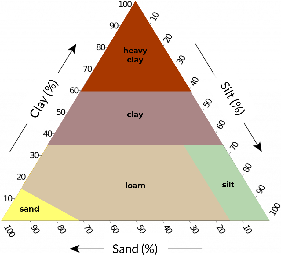
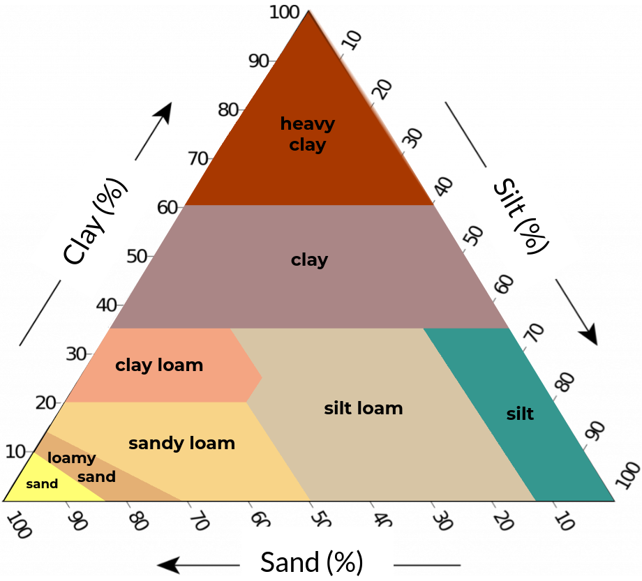
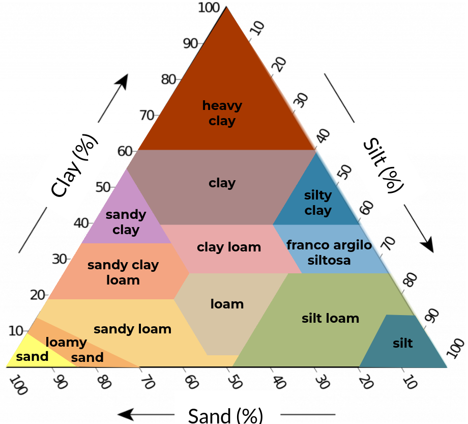
Figure 2. Soil texture classification schemes with five (left), eight (center), and thirteen (right) classes based on clay, silt, and sand content (textural triangle).

Coarse fraction contents were converted to volumetric values using soil and coarse fraction densities. From these data, stoniness maps were generated, identifying depths within the profile (0–100 cm) where coarse fraction volume exceeds the 50% (dominant stoniness) and 90% (extreme stoniness) thresholds. The resulting maps are limited to a depth of 100 cm.

For soil organic carbon (SOC) stock, a single Random Forest model was trained to estimate cumulative stock from the surface to the bottom depth of each layer. To generate the historical series (1985–2024), the model was applied repeatedly by replacing dynamic covariates with each year's respective data, with final predictions for the 30 cm reference depth. This approach captured temporal changes in SOC stock without requiring the chronological year as a numerical predictor.

Point data modeling was performed locally using R and Python, while training and spatial prediction were processed in the cloud via Google Earth Engine. Codes are available under an open license on GitHub (https://github.com/mapbiomas/brazil-soil). Data are available under Creative Commons Attribution CC-BY in the following repositories: https://doi.org/10.58053/MapBiomas/9ORUPF (granulometry), https://doi.org/10.58053/MapBiomas/2LUSVQ (carbon stock), and https://doi.org/10.58053/MapBiomas/1JGPIU (stoniness).

Access the legend code document for MapBiomas Soil Collection 3 here